*******************************************************
QB Rotation Primer
Created: August 16, 1999
Last Modified: June 18, 2000
Toshi Horie <toshiman@uclink4.berkeley.edu>
*******************************************************
Introduction
Rotozoomers are the rage these days in the QB scene. What's a
rotozoomer? It's a graphic effect that rotates and zooms into some
picture. If you remember the spinning logo on the Street Fighter
II game, that was a kind of rotozoomer. If you're interested in the
mathematics behind the code, read on, otherwise, skip to the coding section.
Background
Geometrically speaking, 2D rotozoomers are simply a combination of
rotation and scaling transforms. A rotation transform is a matrix (or set of
formulas) that take a point, and rotate it about some axis, like a clock hand
moves. A scaling transform is a matrix that zooms in or out into a picture.
Let's look at the rotation transform first. You know that the hands of a clock
rotate around the center point. Now imagine those hands moving really fast, like
the Twilight Zone. What shape do they trace out? A circle, right? It turns
out that we can use this fact to help us figure out the formula for rotation.
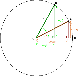
> Figure 1. - Point B is a rotated version of point A.
|
Let's say angle a =
20o. In this figure, you can see Point A is at (cos(a),sin(a)), or
(0.939,0.342). But in polar coordinates, that is (1,a), or
(1,20o) because the radius OA is 1, and it's 20o off the
horizontal +x axis labeled OH.
|
Looking at figure 1, we can see that Point A is in the 2-o'clock position
located at (cos(a),sin(a)). Point B is at the 1 o'clock position, and it is at
(cos(b),sin(b)) in cartesian coordinates. But if you describe the two points in
polar coordinates, as point A is at (1,a) and point B is at
(1,b), it becomes immediately obvious that they only differ in their second
coordinate, which is their angle. So Point B is just Point A rotated by (b-a)
degrees.
So, in polar coordinates, rotation is just
       Rnew = Rold                          .... eq. 1
   Anglenew = Angleold + angle_of_rotation  .... eq. 2
where Rnew is the radius after rotation, and Anglenew is
the angle that the point is at after rotating counter-clockwise
angle_of_rotation degrees.
Ok, but that still doesn't tell us how to rotate a point with coordinates (x,y),
you might think. That's where the sines and cosines come in.
Sines and cosines are not as hard as you think. In terms of polar to cartesian
conversions, they tell you what you have to multiply the radius by to get the x
and y coordinates. Let's say the radius is 1 as in figure 1. Then, if the
angle AOH (the angle created the vector connecting your point and origin, and
the positive x-axis) is 'a' radians, then the x-coordinate of the point is
cosine(a), and the y-coordinate is sine(a). So the formula is:
       x = Radius * COS(a)                .... eq. 3
       y = Radius * SIN(a)                .... eq. 4
Now that we have nice (x,y) coordinates to work with, the rest is easy. You can
see from figure 1, that the coordinates of B are (cos(b),sin(b)). So what does
Point A and Point B differ by? The length of the x-coordinate of point A is
cos(a), and the length of the x coordinate of point B is cos(b). Now you can
subtract the two and find out the difference in the x direction.
       xdifference = (x coordinate of point B) - (x coordinate of point A)
       xdifference =  COS(B) - COS(A)       .... eq. 5 {when radius=1 }
Likewise, the y difference can be found by simple subtraction.
       ydifference = (y coordinate of point B) - (y coordinate of point A)
       ydifference =  SIN(A) - SIN(B)       .... eq. 6 {when radius=1 }
Okay, that was easy, right? Now, we're going to put these results together to
find out the magical equation for rotation.
We'll call the angle between OA and OB "angle c," which is equal to
b-a. We need to rotate A by c radians to get Point B. So we have the equation
       c = b - a                ... eq. 7
       b = a + c                ... eq. 7'
and we have from equation 3 that the coordinates of Point B (= point A after
rotation) given in cartesian coordinates are (Xb,Yb),
where
       Xb = r * SIN(b)  from equation 3
       Xb = SIN(b),     because r = 1
       Xb = SIN(a + c), substituting equation 7'   ... eq. 9


       Yb = r * COS(b)  from equation 4
       Yb = COS(b),     because r = 1
       Yb = COS(a + c), substituting equation 7'   ... eq. 10
Now we need to derive the trigonometric addition identities (equations).
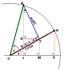
> Figure 2: Diagram for proof of cos(a+c) identity
Derivation of additive trig identities using geometry
- We construct an auxillary line segment BY perpendicular to OA.
This makes length of OY = cos(c) and length of BY = sin(c) because
triangle OBY is a right triangle with hypotenuse |OB| = 1.
- We construct line segment LB to be perpendicular to OM.
- We construct line segment NY to be parallel to OM.
- We construct line segment YM to be perpendicular to OM.
- Now this gives us angle OYN = a because alternate interior angles are congruent.
Also, this gives us the angle NQY = BQY = BQA = 90 - a because it is part of a
right triangle NAQ
- Since vertex Q is part of another right triangle BYQ, angle QBY = 180 - 90 - (90-a) = a
- From Figure 1, you can see that |NL| = |YM| = sin(a) because
it's part of right triangle OAM, and AM is the "opposite" side.
So angle LBY = NYQ = a.
- In right triangle BNY, BN/sin(c) = adj(angle NBY) / hyp(angle NBY) = cos(angle NBY) = cos(a).
Therefore, |NB| = cos(a)*sin(c).
- In right triangle OYM, |YM| / |OY| = opp/hyp = sin(angle YOM) = sin(a).
Combine this with the fact that |NL| = |YM|, you get |NL| = cos(c)*sin(a).
Now we know the coordinates of point B(Xb,Yb):
Xb = cos(a+c) = |LB| = NL + NB = cos(a)*sin(c) + sin(a)*cos(c).
Yb = |OL| = sqrt(|OB2| - |LB|2) = sqrt(1 - |LB|2)
Man, that was a hard proof, but we still have square roots left! We don't want the Yb to contain square roots, because they execute slowly on a computer. Alternate Geometric Proof
We can get |OL| = sin(a+c) through some geometry or algebra:
I'll show the geometric way first, because it's so simple!
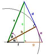
Figure 3: Diagram for proof of sin(alpha+beta) identity
We know from geometry that triangle area = ˝*(base * height). If we
construct altitude c perpendicular to the base formed by joining the line
segments f and g, we can get the left area formula. If we
construct base segments f and g perpendicular to altitude b, we get
the right hand side.
triangle area = triangle area
˝[(c(f+g)] = ˝[b(d+e)]
multiply both sides by two:
c(f+g) = b(d+e) ... eq. 1
by definition,
    sin(alpha) = d/a          ... eq. 2a
    cos(alpha) = b/a          ... eq. 2b
    sin(beta) = e/(f+g)       ... eq. 2c
    cos(beta) = b/(f+g)       ... eq. 2d
    sin(alpha + beta) = c/a   ... eq. 2e
If we multiply eq. 1 by
1/((f+g)*a)
on both sides, we get
c/a = b/a * (d+e)/(f+g)
c/a = d/a * b/(f+g) + b/a * e/(f+g)
Substituting equations 2a,b,c,d,e into the above equation, we get
sin(alpha+beta)= c/a = sin(alpha)cos(beta) + cos(alpha)sin(beta)
That's it, we've proved the sine addition identity! (special thanks to Marduke, who thought of this proof)
Ok, here's the trig and algebra version if you like it that way:
   sin(a+c) = sin(a)cos(c)  + cos(a)sin(c)      ... we just derived this

   sin(a-c) = sin[a+(-c)]
   sin(a-c) = sin(a)cos(-c) + cos(a)sin(-c)
   sin(a-c) = sin(a)cos(c)  + cos(a)*-sin(c)
   sin(a-c) = sin(a)cos(c)  - cos(a)*sin(c)

But if we let a = 90 - a,
   sin[(90-a) - c] = sin(90-a)cos(c) - cos(90-a)sin(c)

Recalling sin(90-x) = cos(x), and cos(90-x) = sin(x), we get
   sin[(90-a) - c] = cos(a)sin(c) - sin(a)cos(c)
   sin[90 - (a+c)] = cos(a)sin(c) - sin(a)cos(c)
          cos(a+c) = cos(a)sin(c) - sin(a)cos(c)
So,
Xb = cos(a+c) = |LB| = cos(a)*sin(c) + sin(a)*cos(c) ...eq. 11
Yb = sin(a+c) = |OL| = cos(a)sin(c) - sin(a)cos(c) ...eq. 12
Now we compare the coordinates of point B and those of point A.
Xa = cos(a)
Ya = sin(a)
and we see that we can substitute Xa whenever we see cos(a), and
Ya whenever we see a sin(a) in equations 11 and 12. Then you get
Xb = Xa * cos(c) - Ya * sin(c)
Xb = Xa * sin(c) + Ya * cos(c)
This is our long-awaited rotation formula for 2 dimensions:
Xrotated = X * COS(angle) - Y * SIN(angle)
Yrotated = X * SIN(angle) + Y * COS(angle)
|
Now the only thing left to do is zoom into that
circle of radius 1 (known as the unit circle) to make this work on all kinds of
points, not just ones that lie on the perimeter of the unit circle. But zooming
is scaling, remember? We'll cover that next.
Scaling in two dimensions is no harder than scaling in one dimension. Just
multiply by the coordinates by scaling factors (a scalar number). So the
formula here is
       XNew = X * scale in x direction         ..... eq. 7
       YNew = Y * scale in y direction         ..... eq. 8
That stretches out the X coordinate by xscale, and the Y coordinate by yscale.
The same formulas are used for the zooming into a picture in a rotozoomer.
Basically, you multiply all your X coordinates by xscale, and all your
Y-coordinates by yscale, and keep increasing xscale and yscale to watch your
picture grow bigger.
DEFINT A-Z
CONST w = 40
CONST h = 30

DIM picture(w, h)
SCREEN 13
'fill the array with pixel colors
'the pattern should look like a rainbow stripe
FOR y = 0 TO h - 1
	FOR x = 0 TO w - 1
		picture(x, y) = x + y + 32
			PSET (x + 280, y + 160), picture(x, y)
	NEXT x
NEXT y

'loop through different scaling factors
'note that as the scales get bigger, there are
'more and more gaps between the colored pixels.
'we will solve this in two ways:
' 1. inverse transformations
' 2. fat pixels with forward transformations
FOR xscale! = .2 TO 5! STEP .2
	FOR yscale! = .2 TO 5! STEP .2
		LOCATE 21, 1
		PRINT USING "xscale=#.#"; xscale!
		PRINT USING "yscale=#.#"; yscale!
		LINE (0, 0)-(xscale! * (w - 1), yscale! * (h - 1)), 15, B
		FOR y = 0 TO h - 1
			FOR x = 0 TO w - 1
				'equation 7 and 8 in action!
				XNew = INT(x * xscale!)
				YNew = INT(y * yscale!)
				PSET (XNew, YNew), picture(x, y)
			NEXT x
		NEXT y
		IF INKEY$ > "" THEN END
	' decrease the flicker by a little
	' and slow down the animation
		WAIT &H3DA, 8: WAIT &H3DA, 8, 8
		WAIT &H3DA, 8: WAIT &H3DA, 8, 8
		WAIT &H3DA, 8: WAIT &H3DA, 8, 8
	' clear the screen for a different scale combination
		LINE (0, 0)-(xscale! * (w - 1), yscale! * (h - 1)), 0, BF
	NEXT yscale!
NEXT xscale!
 |
---> |
 |
| Forward scaling transform |
---> |
Inverse scaling transform |
Type in the program above and run it. You can see that as the scaling factors
get larger (when you zoom in a lot), there are larger gaps in the picture. This
is because I did not bother to fill in those gaps, and because I am using what
is called a forward transformation. A forward transformation just means
that I am transforming the original picture to the screen.
If I transform from the screen back to some pixel on the original picture, I
will be doing a inverse tranformation, and I am guaranteed not to have
"holes" or "gaps" if the picture is big enough. Actually,
you don't have to repeat the picture filling the entire window-- you can make
the parts your picture doesn't cover black or some background color. The code
below shows the double loops required to do a scanline inverse rotation
transformation without tiling.
    REM ...(see ROTATE3 for full code)...
    REM   ...use CLIP (No Tile)...
    angle = 30
    scale = 700
    Ca = c(angle) 'fixed point cosine table
    Sa = s(angle) 'fixed point sine table
    yo = ytop - yd
    FOR y = ytop TO ybottom
        yo = yo + 1
        xo = xleft - xd
        yca = yo * Ca \ scale + yhc
        ysa = yo * Sa \ scale + xhc
        FOR x = xleft TO xright
            xo = xo + 1
            ' note sign reversal in YP due to +Y pointing
            ' downward in screen coordinates.
            xp = xo * Ca \ scale + ysa
            yp = yca - xo * Sa \ scale
            IF (xp>=0 AND xp<=xh AND yp>=0 AND yp<=yh) THEN
                PSET (x, y), model(xp, yp)
            ELSE
                PSET (x, y), 0 :  ' black background
            END IF
        NEXT x
    NEXT y
But if you decide to wrap the picture around infinitely many
times (which is called tiling), you can do it using the MOD
function in BASIC. However, there is
one problem with MOD. If you MOD a negative number by a positive
number, you get a negative number. That is not good when texture coordinates
(coordinates into a 2-D array) have to be positive. There is a work-around,
though. If you DIM your arrays to go from a negative number to a positive
number, you will be ok. A better and faster way is to use AND with a
power-of-2 minus 1 number (like 3,7,15,31,63,127,255,etc). This is equivalent
to MODing by a power of 2 number. For example:
    X  :   -7 -6 -5 -4 -3 -2 -1 +0 +1 +2 +3 +4 +5 +6 +7
X MOD 4:   -3 -2 -1  0 -3 -2 -1  0  1  2  3  0  1  2  3
X AND 3:    1  2  3  0  1  2  3  0  1  2  3  0  1  2  3

61 AND  31 = 29   and   61 MOD 32 = 29 (same result for positive numbers)
-61 AND 31 = 3    but  -61 MOD 32 = -29 (MOD is not what we want for negative)
Here is some code to do tiled inverse rotations like ROTATE3b.

    REM ......Tiled Version (main loops only).......
    REM ......assumes texture is 64x64 pixels.......
    angle = 30
    scale = 700
    Ca = c(angle) 'fixed point cosine table
    Sa = s(angle) 'fixed point sine table
    yo = ytop - yd
    FOR y = ytop TO ybottom
        yo = yo + 1
        xo = xleft - xd
        yca = yo * Ca \ scale + yhc
        ysa = yo * Sa \ scale + xhc
        FOR x = xleft TO xright
            xo = xo + 1
            ' note sign reversal in YP due to +Y pointing
            ' downward in screen coordinates.
            xp = xo * Ca \ scale + ysa
            yp = yca - xo * Sa \ scale
            PSET (x, y), model(xp AND 63, yp AND 63)
        NEXT x
    NEXT y
To fix the problem with the "gaps" and "holes" that occur
when rotozooming with the standard rotation formula, we use a technique called
reverse or inverse rotation transformations. The idea is simple: instead
rotating points on the figure and ending up somewhere on the screen, we do the
opposite: rotate the screen coordinates backwards, so that they land on the
model somewhere. We already did a similar thing with the scaling transform.
In our QB program, it amounts to changing the point number loop to a x,y loop, and using this formula:
Xrotated = Xscreen * COS(angle) + Yscreen * SIN(angle)
Yrotated = - Xscreen * SIN(angle) + Yscreen * COS(angle)
|
The formula comes from substituting -angle in place of angle, and
using some negative angle trig identities to clean things up.
When we rotate things around the origin (0,0), we can use the pure rotation or
inverse rotation formula as-is, but when we usually want to move things around
so that our model coordinates end up being 0 to some positive number, because
they are array coordinates. In order to do this, you have to do a translation
transform, the regular rotation transform, then another translation tranform to
put those points where they should land.
      R(angle with different center) = Translation1 * R(angle) * Translation2

             where * is the composition operator
|
Here is a QB code fragment that does this.
    REM ......CENTER of ROTATION CHANGE demo........
    REM ......tiled sprites, untested code.......
    REM ......assumes texture is 64x64 pixels.......
    angle = 30
    scale = 700
    xcenter = 35
    ycenter = 27
    Ca = c(angle) 'fixed point cosine table
    Sa = s(angle) 'fixed point sine table
    yo = ytop - yd
    FOR y = ytop TO ybottom
        yo = yo + 1
        xo = xleft - xd  'translation 1
        yca = yo * Ca \ scale + ycenter
        ysa = yo * Sa \ scale + xcenter
        FOR x = xleft TO xright
            xo = xo + 1
            ' note sign reversal in YP due to +Y pointing
            ' downward in screen coordinates.
            xp = xo * Ca \ scale + ysa
            yp = yca - xo * Sa \ scale
            PSET (x, y), model(xp AND 63, yp AND 63)
        NEXT x
    NEXT y
This topic falls under optimizations a bit too, because if you use this algorithm,
your rotozoomer will go faster. The Digital Difference Analyzer (DDA) is based on the
idea that if you go in a straight line in screen coordinates, you will also
go in a straight line in the image sprite coordinates. This straight line has a
constant slope, which is equal to the slope of all lines parallel to it. This slope,
which we will call m1 has two components: the d1x and d1y
components. Everytime we move along the rotated line, we add d1x and
d1y to u and v, our image sprite coordinates. When we move down a row in
the screen coordinates (Y=Y+1), we move it another direction that we'll call m2,
that are made up of two components, d2x and
d2y. So to rotate an image using DDA, all you need is two nested
loops with two adds each. Since there are no multiplications needed in the
loops, it runs very fast.
You can check the DDA source code here.
Sinus Table Size
Some people were lost when I changed the table size in ROTATE3b. Here is the generalized sine and cosine table
calculation code. You'll find that it works if you plug in tsize=360, and it
works for any other even integer value, too. What it does is divide the angles
for a full 360 degree rotation into tsize steps. It works because the step side
is calculated correctly using deg2bin# = 2 * pi# / tsize, and the first FOR loop
calculates the sine and cosine values for that every angle up to 180 degrees,
and the second loop "flips" those values so that you get the correct
sines and cosines for angles between 180 and 360 degrees.
CONST tsize = 128: 'sine lookup table size
scale = 512:       'fixed point scaling factor

DIM c(tsize): DIM s(tsize)

'set up sinus tables
pi# = 3.1415926535#
deg2bin# = 2 * pi# / tsize
PRINT "Calculating sine/cosine tables..."
FOR theta = 0 TO (tsize\2-1)
    s(theta) = CINT(SIN(theta * deg2bin#) * scale)
    c(theta) = CINT(COS(theta * deg2bin#) * scale)
NEXT
FOR theta = (tsize\2) TO (tsize-1)
    s(theta) = -s(theta - (tsize\2-1))
    c(theta) = c((tsize-1) - theta)
NEXT
If you can think of a better explanation, please email me.
Optimizations in general are a good thing. Algorithmic
optimizations that improve the speed and/or memory usage of the program by
more than a constant factor is definitely worth doing. On the other hand, it's
easy to get caught up in low-level optimizations that amount to only a few
percent increase in program speed, and lose sight of major good
optimizations that work on any machine.
Optimizations often make the code difficult to understand, and lead to
insidious bugs. So it's a good idea to document why you made the
optimization, the original algorithm (so you can test if your optimized version
still works correctly) and all the side-effects and trade-offs of
the optimization. For example, precalculation has the trade-off that more
memory is used in exchange for faster program execution. Precalculated sine
tables have the side effect that you can get a SUBSCRIPT OUT OF RANGE error if
you don't wrap around the angle, while the SIN function lets you use any angle.
If you use fixed point INTEGER math, you get the side effect of "shaky" or
"hairy textures" unless you use more bits of precision and prestep
your texture starting coordinates at each row.
In many programs, there are functions that get called very often. One
programmer has even said, "Most programs spend 95% of their time in 5% of
the code." These pieces of code are called inner loops or
hotspots, and are the prime candidates for optimization. In the case of
QB games, the inner loop is usually the rendering loop or keyboard polling loop.
In our rotozoomer, the inner loop is obviously the inner pixel plotting loop.
Let's take a look at the unoptimized loop for the inverse rotation transform algorithm.
	FOR y = ytop TO ybottom
		FOR x = xleft TO xright
			yo = yd - y
			xo = x - xd
			xp =  xo * COS(angle * deg2rad#) / scale# + yo * SIN(angle * deg2rad#) / scale#
			yp = -xo * SIN(angle * deg2rad#) / scale# + yo * COS(angle * deg2rad#) / scale#
			PSET (x, y), model(xp AND 63, yp AND 63)
		NEXT x
	NEXT y
The first thing I see is the long expression for xp and yp in the inner loop.
I'm talking about this:
	xp =  xo * COS(angle * deg2rad#) / scale# + yo * SIN(angle * deg2rad#) / scale#
	yp = -xo * SIN(angle * deg2rad#) / scale# + yo * COS(angle * deg2rad#) / scale#
I notice that the last expression on both lines are constant in the inner loop,
because they depend on yo, scale# and angle only, which don't change when the x
changes. So we can take them out of the inner loop, and we get this:
	FOR y = ytop TO ybottom
		'we precalculated the variables that depend on y outside the inner loop
		yo = yd - y
		ysa# = yo * SIN(angle * deg2rad#) / scale#
		yca# = yo * COS(angle * deg2rad#) / scale#
		FOR x = xleft TO xright
			xo = x - xd
			xp = xo * COS(angle * deg2rad#) / scale# + ysa#
			yp = -xo * SIN(angle * deg2rad#) / scale# + yca#
		PSET (x, y), model(xp AND 63, yp AND 63)
		NEXT x
	NEXT y
Next we can precalculate the sine and cosine of each integer degree angle. This
will get rid of an expensive (slow) multiply and FPU calculation of SIN and COS
in the inner loop.
DIM cosine#(360)
DIM sine#(360)
FOR angle = 0 TO 359
	cosine#(angle) = COS(angle * deg2rad#)
	sine#(angle) = SIN(angle * deg2rad#)
NEXT angle

'zoom in and rotate the model
DO
	angle = (angle + 1) MOD 360 'rotate counter-clockwise by 1 degree
	scale# = scale# + .05
	LOCATE 2, 10: PRINT angle; "degrees"
	k$ = INKEY$: IF k$ = esc$ THEN EXIT DO
	FOR y = ytop TO ybottom
		yo = yd - y
		ysa# = yo * sine#(angle) / scale#
		yca# = yo * cosine#(angle) / scale#
		FOR x = xleft TO xright
			xo = x - xd
			xp = xo * cosine#(angle) / scale# + ysa#
			yp = -xo * sine#(angle) / scale# + yca#
		PSET (x, y), model(xp AND 63, yp AND 63)
		NEXT x
	NEXT y
LOOP
END
Run it now and see how much faster it is!
Now what can we do? Fixed Point! But fixed point is tricky, I warn you.
My computer graphics teacher explains the axiom of fast computer graphics,
"Don't do anything you don't have to during runtime; precalculate as much as
possible!"
Here's an example of a good precalc in QuickBasic.
DIM sins(128) AS INTEGER
DIM coss(128) AS INTEGER
FOR s = 0 TO 128
    sins(s) = 256 * SIN(s * PI / 64) * (COS(s * PI / 64) + 1.5)
    coss(s) = 256 * COS(s * PI / 64) * (COS(s * PI / 64) + 1.5)
NEXT s
With the sins() and coss() tables set up, you can now get complex sinusoidal
motion, just by doing a table look-up like
  FOR S = 0 TO 127
       PSET(sins(s),coss(s))
  NEXT S
Precalculated arrays of this sort are called Lookup Tables or LUTs,
and can speed up calculations by a lot if used cleverly.
Computers were originally designed to be adding machines. So they were designed
to add a fixed number of digits very quickly*. For this and a number
of other technical reasons, INTEGER calculations are faster than FLOATing point
calculations on many personal computers. We can take advantage of this in
BASIC, by working in fixed point, just like a cash register. In a cash
register, there are two digits after the decimal point, never more, never less.
Ok, what if we moved the decimal point two digits to the right? Then we're
dealing with cents, and we'll always get INTEGER values. Ok, not always, but we
round off to the nearest cent anyways, right? (To do that, you just move the
decimal point one further to the right, but don't use it unless you need to do
rounding.)
To do fixed point in QuickBasic, you multiply lots of floating point numbers by
a big integer (called the scaling factor), and save the results in a
precalculated look-up table, then in your inner loop, you do some arithmetic on
the values in the look-up table, then right before you use that number, divide
the value by the scaling factor. (in C++ or ASM, logical binary shifts do the
dividing part even faster).
Let's look at an example in decimal:
Say you want to represent 374.6031 in 5.2 fixed point (think of it as #####.##.)
It's really easy, you just fill in the hash marks and get 374.60, represented in cents as 37460. Notice we just moved the decimal point to the right by two to make it an even integer.
Now here's a hexadecimal version:
Say you wanted to convert 0x374.6031 to real 5:2 FIXED POINT. Since there's only room for 2 hexadecimal digits after the decimal point, you get 0x374.60.
You can just multiply this by 0x100 to make it the even integer that
represents this FIXED POINT quantity. Conversely, you can <<2 to
get the scaled up version, and >>2 to scale back down.
Here's an example where we can get an idea of how fast fixed point math is
compared to floating point!
DEFINT A-Z   'we want QB to use INTEGERs for SPEED!
scale = 256  'scaling factor
deg2rad# = .01745329#
PRINT "Calculating sinus tables..."
DIM c(360), s(360)
FOR t = 0 TO 359
	c(t) = COS(t * deg2rad#) * scale    ' scale up!
	s(t) = SIN(t * deg2rad#) * scale    ' scale up!
NEXT

'let's use some fixed point
scale2 = scale \ 16

tstart# = TIMER
FOR t = 0 TO 359
	PRINT c(t) \ scale2, s(t) \ scale2  ' scale down! (a little)
NEXT t
tend# = TIMER
tfast# = tend# - tstart#

'try the slow floating point version
scalex = scale \ scale2
tstart# = TIMER
FOR t = 0 TO 359
	PRINT INT(COS(t * deg2rad#) * scalex), INT(SIN(t * deg2rad#) * scalex)
NEXT t
tend# = TIMER
tslow# = tend# - tstart#

'display competition results
PRINT USING "   Fixed Point took ##.### secs."; tfast#
PRINT USING "Floating Point took ##.### secs."; tslow#
PRINT USING "Fixed point was ####% faster"; (tslow# - tfast#) * 100 / tslow#
Even on a Pentium III, where floating point math is VERY fast, fixed point won
this competition by a 12% margin.
More to come....
Please give me credit for the ROTATEn.BAS examples if you use my code. --Toshi
You can to refer back to the Math Tricks or Optimization section if you don't see what I'm doing.